Why L1 norm creates Sparsity compared with L2 norm
Distance is calculated between points and Norm calculated between vectors
What is Norm?
In simple words, the norm is a quantity that describes the size of a vector, something that we can represent using a set of numbers as you might already know that in machine learning everything is represented in terms of vectors. In this norm, all the components of the vector are weighted equally.
let’s take vector ‘a’ that contains two elements X1 and X2. We can represent the features of vector ‘a’ in two-dimensional (2d).
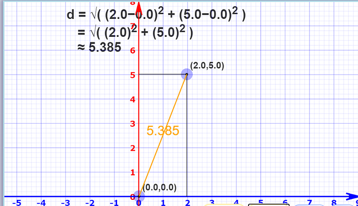
a = (2,5) and O(0,0)
- L2 Norm / Euclidean distance
Let’s calculate the distance of point a from the origin (0,0) using the l2 norm, which is also known as Euclidean distance.
Euclidean distance =||X1 -X2 ||2 ~ Sqrt(( ∑ i = 1 to k (x1i -x2i)²))


2. L1 Norm / Manhattan distance
We can also calculate distance using another way to measure the size of the vector by effectively adding all the components of the vector and this is called the Manhattan distance a.k.a L1 norm.
Manhattan distance = ||X1-X2||1 ~ (summation(abs(X1i-X2i)))
Manhattan Distance [{a, b}, {x, y}] = Abs [a − x] + Abs [b − y]
[{0,0} , {2,5}] = |0–2| + |0–5| = |-2|+|-5| = 2+5 = 7
The generalize equation of ln norm is the nth root of the summation of all components to their nth powers.
3. L-infinity norm


Gives the largest magnitude among each element of a vector.
Having the vector X= [-6, 4, 2], the L-infinity norm is 6.
In the L-infinity norm, only the largest element has any effect. So, for example, if your vector represents the cost of constructing a building, by minimizing the L-infinity norm we are reducing the cost of the most expensive building.
The behavior of the norms
The plot describes the behavior of every vector that has an L1 norm equal to 1. Every point on the circumference of the square is a vector with L1 norm = 1 but what happens when we do it for the l2 norm? It becomes a circle and it’s actually easy to guess because in the equation of the circle in 2d there are square terms right and in the formula of l2 norm there are squares
so it makes sense right every point on the circumference of the circle has l2 norm as one let’s see what happens to the circle as we increase n.

we can clearly see that as we increase the order the shape approaches a square but wait how did I even calculate the L infinity norm well I just took the
limit of the formula as n approaches infinity it turns out that L infinity is just the maximum component of the vector now that we have a very good
understanding of the norms.
Where norms are used the most common?
- Mean Squared Error
- Ridge Regression Constraint
- Lasso Regression Constraint
Mean Squared Error: The mean squared error (MSE) or mean squared deviation (MSD) of an estimator (of a procedure for estimating an unobserved quantity) measures the average of the squares of the errors — that is, the average squared difference between the estimated values and the actual value.

The error cost function is the sum of the squared differences between ground truths and predictions are nothing but the l2 norm of the resultant vector formed by subtracting the vector of predictions from the vector of ground truths.
Ridge Regression Constraint :
we put a constraint on the weights and the constraint says nothing but the l to the norm of the weight vector should be greater than or equal to some positive value visually the optimized weight vector should lie outside the red circle.


Lasso Regression Constraint :
If we talk about lasso regression then the constraint becomes l1 norm and in this case, the optimized weight vector should lie outside the red square.


Why L1 norm creates Sparsity?
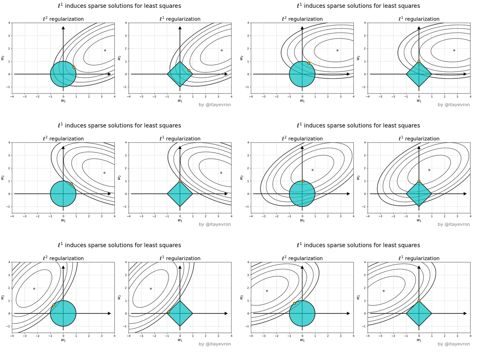
We gonna have a quick tour on why the l1 norm is so useful for promoting sparse solutions to linear systems of equations. The reason for using the L1 norm to find a sparse solution is due to its special shape. It has spikes that happen to be at sparse points. Using it to touch the solution surface will very likely to find a touch point on a spike tip and thus a sparse solution.

The above figure is the geometric perspective on sparsity and the L1 norm and L2 norm.

The solid blue areas are the constraint regions |β1|+|β2| ≤ r and β1² + β2² ≤ t², respectively, while the res ellipses are the contours of the least squared error functions.
The β^ is the unconstrained least squares estimate. The red ellipses are (as explained in the caption of this Figure) the contours of the least-squares error function, in terms of parameters β1 and β2. Without constraints, the error function is minimized at the MLE β^, and its value increases as the red ellipses out expand. The diamond and disk regions are feasible regions for lasso (L1) regression and ridge (L2) regression respectively. Heuristically, for each method, we are looking for the intersection of the red ellipses and the blue region as the objective is to minimize the error function while maintaining feasibility.
That being said, it is clear to see that the L1 constraint, which corresponds to the diamond feasible region, is more likely to produce an intersection that has one component of the solution is zero (i.e., the sparse model) due to the geometric properties of ellipses, disks, and diamonds. It is simply because diamonds have corners (of which one component is zero) that are easier to intersect with the ellipses that extending diagonally.
Intuitions of L1 Norm and L2 Norm.
Why we use norms? In complex machine learning models, Overfitting occurs when your model learns too much from training data and isn’t able to generalize the underlying information.
Cross-validation, Remove features, Early stopping, Regularization are some processes used to prevent overfitting. Let’s focus on L1 and L2 regularisation
The main intuitive difference between the L1 and L2 regularization is that L1 regularization tries to estimate the median of the data while the L2 regularization tries to estimate the mean of the data to avoid overfitting.


In optimization formulation for comparison Loss and λ can be ignored as they are the same for both L1 and L2 regularization.
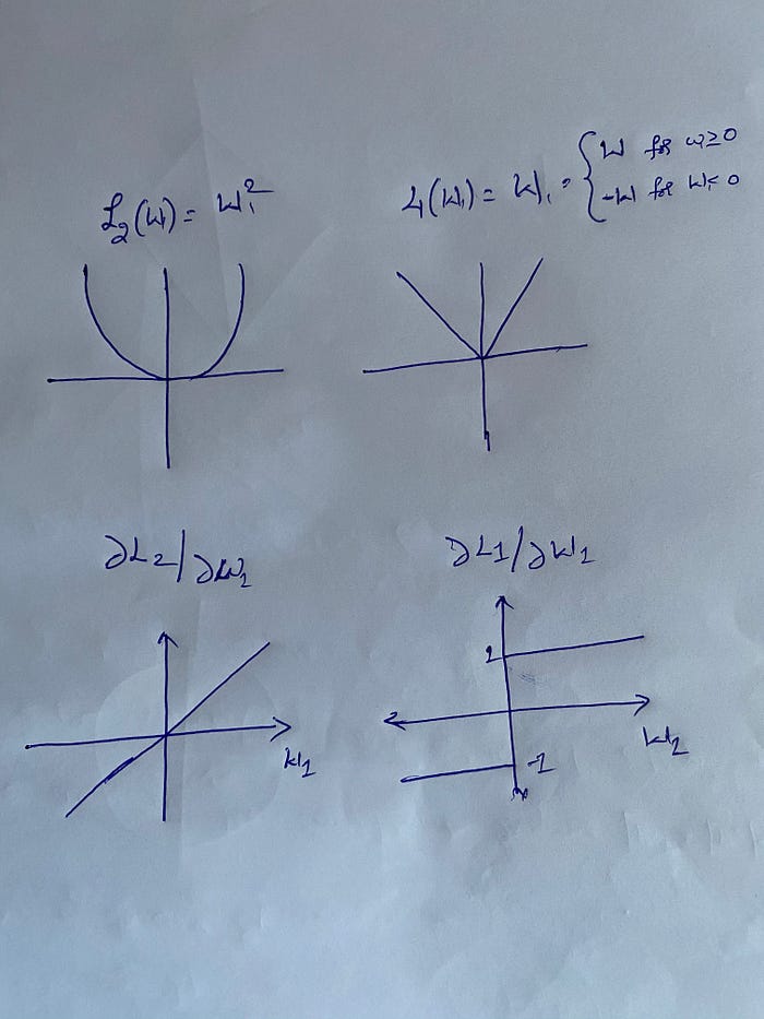
L2 has min(W) for (W1²+W2²+………Wd²) ==> this is a parabola.
L1 has min(W) for (|W1|+|W2|+…|Wd|) ==> V shaped vector.
L2(W) = W1² ==> DL2/DW1 = 2*W1; derivative is a straight line.
L1(W) = W1 ==> DL1/DW1 = +1 or -1 ; derivate of step function.
W1@(j+1) = W1(j)-r*(DL/DW1)@(W1j) ; r → learning rate.
Let W1 is a positive number
For L2, W1@j+1 = W1@j -r*(2*W1@j) ; For L1, W1@j+1 = W1@j-r*1
L2 updates occur less when compared to L1 updates as we reach closer to optimum, that is the rate of convergence decreases because L2 regularization we have 2*W1*r which is less than r.

This happens because the L1 derivate is constant and the L2 derivative not constant.
For example: W = 5 and r = 0.05
L2 = W-(r*2W)= 5-(0.05*2*5) = 5-(0.05*10) = 5-0.5 = 4.5
Iteration 2 : 4.5-(0.05*2*4.5) = 4.5–0.45 = 4.05
L1 = W-(r*1) = 5-(0.05*1) = 5-0.05 = 4.95
Iteration 2 :4.95-(0.05*1) = 4.95–0.05 = 4.90
The chance of weights reaching zero (0) is more for L1 as the derivative is constant and independent of the previous weight value while L2 has derivatives reducing as the derivative is dependent on the previous iteration weight value which is converging to optimal.
Reference:
https://www.youtube.com/watch?v=FiSy6zWDfiA
https://www.youtube.com/watch?v=76B5cMEZA4Y&t=262s
https://towardsdatascience.com/intuitions-on-l1-and-l2-regularisation-235f2db4c261
https://stats.stackexchange.com/questions/45643/why-l1-norm-for-sparse-models